pacman::p_load(ggiraph, tidyverse, ggplot2,dplyr,funModeling,ggpubr, plotly )Take-home Exercise 2
1. Overview
The task Take-home Exercise 2 is to select one of the Take-home Exercise 1 prepared by our classmate, critic the submission in terms of clarity and aesthetics,prepare a sketch for the alternative design by using the data visualisation design principles and best practices we had learned in Lesson 1 and 2, and remake the original design by using ggplot2, ggplot2 extensions and tidyverse packages.
2. Installing and loading R packages
Two packages will be installed and loaded. They are tidyverse and ggiraph.
3. Importing data
population <- read_csv("data/respopagesextod2022.csv")Rows: 100928 Columns: 7
── Column specification ────────────────────────────────────────────────────────
Delimiter: ","
chr (5): PA, SZ, AG, Sex, TOD
dbl (2): Pop, Time
ℹ Use `spec()` to retrieve the full column specification for this data.
ℹ Specify the column types or set `show_col_types = FALSE` to quiet this message.4. Visualization Critique
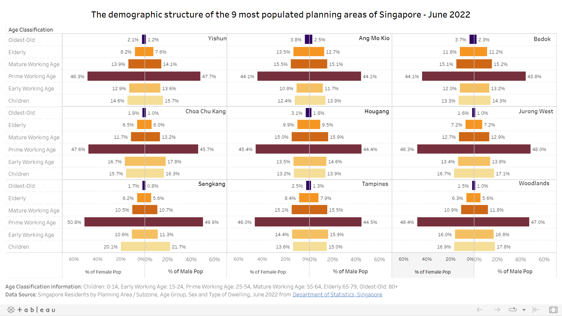
4.1 Original design
The following is the age-sex pyramid provided by my classmate in this take-home exercise 1 and it will be reviewed and remade in terms of clarity and aesthetics.
4.2 Clarity
4.2.1 Graphical Integrity: Show Me the Truth
The better way for define the age group segmentation should be 0-4, 5-9, etc, and not “children”,“early working age”, etc. The reason is “children”,“early working age”, etc is too general, it will mask out age segmentatio signal.
4.2.2 Visualising the Right Data
Absolute values will reveal more interesting patterns than the derived values. From the derived values which is population in percentage, we will not know what is the number of female and male population difference from the 9 most populated planning areas.
4.2.3 Reference line
In the remake, the reference line is added which is the avg population (sum of total population divided by 9 planning areas/19 age groups/2 genders).
4.2.4 interactive function
Add on interactive function into the chart to show the population numbers when move cursor.
4.3 Aesthetics
4.3.1 Application of pre-attentive principle
Colours. The original age-sex pyramid used one color for two genders. However, this display does not show a clear comparison betewwn male and female population. It does not help user to distinguish the genders from the 1st attention. . It’s suggested to choose two different colors to indicate the two different genders in this visualization.
4.3.2 X-Axis Title & Labels
The population number is large. It’s good to show number in the unit of thousand With the aid of the newly added x-axis title and labels, it makes it easier for users to read and interpret this visualization. The X-axis labels will be converted to positive values because population should be positive values.
4.3.3 Caption
The caption to mention the data source for this visualization has also been included at the bottom in a clean manner.
5. Visualization Remake step by step
Calculate total population count by planning area
pop_pa <- population %>%
  select(PA,AG,Sex,Pop) %>%
  group_by(PA) %>%
  summarise(totalPop = sum(Pop))
Sort planning areas by population
pop_sorted <- pop_pa[order(pop_pa$totalPop, decreasing = TRUE), ]Select top 9 planning areas by population
pop_filtered <- head(pop_sorted, 9)Filter the raw dataset according to the top 9 planning areas by population
pop_pa_filtered <- population %>%
  filter(PA %in% pop_filtered$PA)
aggregate data by planning areas, age group and sex
Pop_pa_age_sex <- aggregate(Pop ~ PA + AG + Sex, data = pop_pa_filtered, FUN = sum)Sort dataset by top 9 planning areas and age group
verify the age groups
freq(data=Pop_pa_age_sex ,
     input = 'AG')
Warning: The `<scale>` argument of `guides()` cannot be `FALSE`. Use "none" instead as
of ggplot2 3.3.4.
ℹ The deprecated feature was likely used in the funModeling package.
Please report the issue at <https://github.com/pablo14/funModeling/issues>.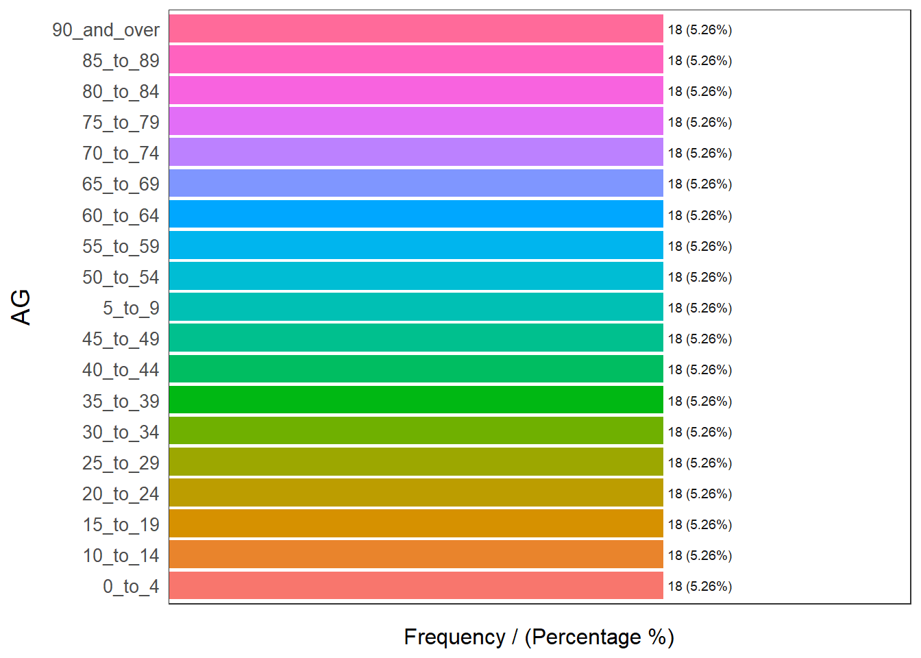
            AG frequency percentage cumulative_perc
1       0_to_4        18       5.26            5.26
2     10_to_14        18       5.26           10.52
3     15_to_19        18       5.26           15.78
4     20_to_24        18       5.26           21.04
5     25_to_29        18       5.26           26.30
6     30_to_34        18       5.26           31.56
7     35_to_39        18       5.26           36.82
8     40_to_44        18       5.26           42.08
9     45_to_49        18       5.26           47.34
10      5_to_9        18       5.26           52.60
11    50_to_54        18       5.26           57.86
12    55_to_59        18       5.26           63.12
13    60_to_64        18       5.26           68.38
14    65_to_69        18       5.26           73.64
15    70_to_74        18       5.26           78.90
16    75_to_79        18       5.26           84.16
17    80_to_84        18       5.26           89.42
18    85_to_89        18       5.26           94.68
19 90_and_over        18       5.26          100.00
order the age groups
Pop_pa_age_sex$AG[which(Pop_pa_age_sex$AG=="0_to_4")] <-"00_to_04"
Pop_pa_age_sex$AG[which(Pop_pa_age_sex$AG=="5_to_9")] <-"05_to_09"
Derived the population in thousand and avg population in thousand
pop_final <- Pop_pa_age_sex %>%

  mutate(Pop_2=round(Pop/1000,2))%>%
  mutate(Avg=round(sum(Pop)/1000/9/19/2,2))%>%
  arrange(PA, AG)
Create the age_sex_pyramid
age_sex_pyramid <- ggplot(data=pop_final,aes(x=AG,fill=Sex)) +
  theme_bw() + ## change background color to white
  geom_bar(data=subset(pop_final,Sex=="Females"),stat='identity',aes(y=Pop_2)) +
  geom_bar(data=subset(pop_final,Sex=="Males"),stat='identity',aes(y=Pop_2*(-1)))  +
  scale_y_continuous(breaks=seq(-20,20,5),labels=abs(seq(-20,20,5))) +
  facet_wrap(~ PA)+
  coord_flip()+
  theme_bw() +
  scale_fill_manual(values = c("Males" = "blue",
                               "Females" = "red")) +


  labs(x = "Age Group",
       y = "Population(in thousand)",
       title = "Singapore Population Pyramid by age&sex from top 9 Planning Areas in June 2022",
       subtitle = "Top 9 Planning Areas by Population, 2022",
       caption = "Data Source: https://www.singstat.gov.sg/find-data/search-by-theme/population/geographic-distribution/latest-data")+

    theme(plot.title = element_text(hjust=0.5, size=14),
          plot.subtitle = element_text(hjust = 0.5,size = 8),
          legend.title = element_text(size=10),
          legend.text = element_text(size=8),
          axis.text = element_text(face="bold"),
          axis.ticks.x=element_blank(),
          axis.text.x = element_text(angle = 0),
          axis.title.y=element_text(angle=0))

age_sex_pyramid_final <-age_sex_pyramid + geom_hline(yintercept = pop_final$Avg,linetype="dotted", color = "black") + geom_hline(yintercept = -(pop_final$Avg),linetype="dotted", color = "black")+

  geom_text(aes(0,Avg,label = 'Avg', vjust = -1))+
  geom_text(aes(0,-Avg,label = 'Avg', vjust = -1))

ggplotly(age_sex_pyramid_final)